Real Time Power Quality Monitoring Using Multimodal Fusion

Table of Contents

1. Abstract

2. Introduction

3. Problem Statement and Objectives

4. Literature Review

5. Standards and Regulatory Context

6. Theoretical Background

7. System Architecture Overview

8. Hardware Design

9. Firmware — Teensy 4.1 Embedded Software

10. Signal Processing and Feature Extraction Pipeline

11. Deep Learning Model

12. Dataset Generation

13. Training Procedure and Evaluation

14. Experimental Plan and Demo Setup

15. Hardware Design Audit — All Issues, Root Causes, and Fixes

16. Complete Bill of Materials

17. Complete Wiring Diagram and Connections

18. Safety Guidelines

19. Implementation Timeline

20. Known Limitations and Future Extensions

21. References

1. Abstract

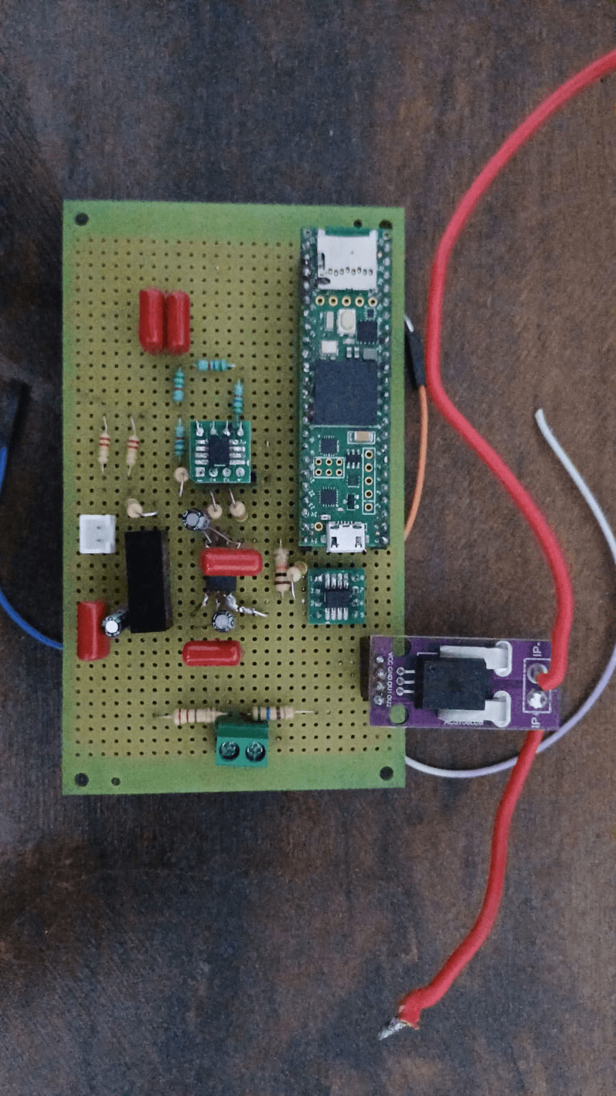
This project presents the complete design and implementation of a low-cost, hardware-enabled, real-time system for detection and classification of power quality (PQ) disturbances in low-voltage (LV) 230 V / 50 Hz industrial networks. The hardware sensing node uses a Texas Instruments AMC1301 reinforced isolated differential amplifier preceded by a precision 2.2 MΩ / 560 Ω resistor voltage divider to safely measure the 230 V mains waveform, and an Allegro ACS758LCB-050B Hall-effect current sensor to simultaneously capture load current. Both analog channels are sampled synchronously at 5 kHz using the dual-ADC simultaneous hardware mode of the PJRC Teensy 4.1 microcontroller (Cortex-M7 @ 600 MHz), giving exactly N = 500 samples per 50 Hz cycle — a deliberate design choice that places every harmonic (50, 100, 150, … Hz) on an exact integer FFT bin, eliminating spectral leakage entirely for stationary periodic signals.

In the current repo state, the production runtime is a Raspberry Pi kiosk workflow. By default, the Teensy computes the canonical 298-element feature vector on-device, packs the inference inputs into a model-ready serial frame, and streams that payload over USB to the Pi. The Pi runtime consumes the packed tflite frame, reconstructs the three inference tensors X_wave, X_mag, and X_phase, and runs the deployed artifacts/models/pqm_multilabel_model.tflite model while driving a touch dashboard, event log, and replay/debug tooling. Legacy raw-frame and 282-feature compatibility paths remain in the repository for capture, parity testing, and fallback debugging, but they are no longer the active production contract.

Four model variants (M1 through M4) remain the research lineage used to quantify the contribution of phase information, while the checked-in integration repository is centred on the exported TFLite inference artifact and the 298-feature deployment contract. Domain adaptation via fine-tuning on real hardware samples remains part of the ML plan, and the current frontend bill of materials in this report places the sensing hardware cost at approximately ₹791 rather than under ₹700.

The project’s core scientific contribution is demonstrating that harmonic phase angles carry load-type-specific signatures that are statistically distinct even when harmonic magnitudes are nearly identical — and that a deep learning model trained on phase-aware features can exploit this information to improve classification accuracy by 1–3% overall and substantially more for hard-to-distinguish class pairs.

2. Introduction

2.1 The Power Quality Problem in Modern Industry

Modern industrial and commercial facilities depend heavily on power-electronic equipment: variable-frequency drives (VFDs) for pumps, fans, and CNC machines; rectifier-front-end uninterruptible power supplies (UPS); switched-mode power supplies (SMPS) in computers, servers, and LED drivers; and increasingly, electric vehicle (EV) chargers. All of these devices are nonlinear loads: unlike a simple resistive heater or incandescent lamp, they draw current in short, sharp pulses rather than as a smooth sinusoidal waveform.

The governing physics is straightforward. The utility provides a nominally sinusoidal voltage at 230 V RMS, 50 Hz. A linear load — one whose impedance is constant — draws a proportional sinusoidal current. A nonlinear load has a time-varying impedance (e.g., a diode bridge only conducts when the supply voltage exceeds the DC rail voltage), so it draws a current whose shape is not sinusoidal.

By Fourier’s theorem, any periodic waveform is the superposition of sinusoids at the fundamental frequency and its integer multiples — the harmonics. For a 50 Hz fundamental: the 2nd harmonic is at 100 Hz, the 3rd at 150 Hz, the 5th at 250 Hz, and so on. Nonlinear loads inject harmonic currents into the network; those currents flow through the finite impedances of cables, transformers, and busbars, creating harmonic voltage drops that distort the voltage seen by every load on the same network.

The consequences in a real industrial facility are significant and costly:

Transformer overheating: Harmonic currents increase copper losses (I²R) and core losses (eddy current losses scale with f²). A transformer carrying rated fundamental current plus significant harmonic content runs hotter than nameplate ratings indicate and fails prematurely.

Neutral conductor overloading: In a balanced three-phase system, fundamental-frequency phase currents cancel in the neutral. However, triplen harmonics (3rd, 9th, 15th — multiples of 3) do NOT cancel; they add arithmetically. A neutral sized for imbalance current may carry 1.7× the phase current when triplen harmonics are dominant — a fire hazard.

Capacitor bank failures: Power factor correction capacitors present a low impedance path to harmonic currents. The resulting high harmonic currents cause dielectric overheating, stress, and early failure. Resonance between the capacitor bank and network inductance at a harmonic frequency can amplify that harmonic by 5–10×.

PLC and sensitive electronics malfunction: Harmonic voltage distortion causes microcontroller-based equipment to malfunction, reset unexpectedly, or produce measurement errors — particularly in precision measurement instruments whose ADC reference is derived from the mains.

Meter errors: kWh meters calibrated for sinusoidal waveforms over-read or under-read when harmonics are significant, leading to billing disputes.

Motor derating: Negative-sequence harmonics (5th, 11th, 17th) create counter-rotating magnetic fields in AC induction motors, increasing losses, reducing torque, and requiring derating. At 5% 5th-harmonic voltage, derating to 90% of nameplate rating is typically required.

2.2 Why Monitoring Matters

The first step in addressing a power quality problem is measuring it accurately. Without quantitative data about the type, magnitude, duration, frequency of occurrence, and timing of disturbances, it is impossible to:

• Determine whether the disturbance originates from local loads (user-side) or the utility grid (supply-side) — critical for deciding who bears the cost of mitigation.

• Size and specify appropriate mitigation technology (passive harmonic filters, active harmonic filters, line reactors, isolation transformers, or dynamic voltage restorers).

• Verify compliance with applicable standards (IEEE 519-2022, EN 50160, IEC 61000-3-2) before and after mitigation.

• Monitor for gradual degradation that may precede equipment failures (predictive maintenance).

• Build an event log for insurance claims or utility negotiations.

2.3 The Gap: Phase Information is Universally Ignored

Conventional power quality monitors — including those meeting IEC 61000-4-30 Class A requirements (Hioki PQ3198, Fluke 435-II, Dranetz HDPQ) — measure harmonic magnitudes and total harmonic distortion (THD) with high accuracy. However, virtually all standard instruments and published research methods focus exclusively on magnitude spectra. The phase angles of individual harmonic components are discarded.

This is a meaningful loss of information. The phase structure of a harmonic spectrum is physically determined by the mechanism generating those harmonics, not random:

• A 3rd harmonic generated by a single-phase bridge rectifier (SMPS) has a phase relationship to the fundamental concentrated near ±45° because it is produced by the capacitor charge pulse at the voltage peak.

• A 3rd harmonic from a transformer saturating on the voltage peak has phase concentrated near ±90° (near the voltage zero crossing) because saturation occurs when flux — the integral of voltage — reaches its peak.

• The 5th harmonic in a 6-pulse VFD rectifier has a fixed phase relationship to the firing angle α; the ratio of 5th-to-7th harmonic phases encodes the rectifier’s operating point.

• Two scenarios can produce identical THD values but entirely different phase structures, making them impossible to distinguish from magnitude alone.

This project explicitly exploits harmonic phase information by combining it with magnitude features in a deep learning classifier designed to improve discrimination between power quality disturbance types and harmonic sources.

2.4 Project Motivation and Scope

This project targets an intelligent, low-cost, phase-aware PQ monitor for academic demonstration, laboratory use, and small-scale industrial deployment. The current frontend bill of materials is approximately ₹791 for the sensing frontend — compared to commercial PQ analysers costing ₹50,000 to ₹5,00,000. The project demonstrates:

1. That publication-quality harmonic measurements (amplitude AND phase) are achievable with commodity components when the electronics are designed carefully.

2. That incorporating phase information into a deep learning classifier measurably improves classification accuracy versus magnitude-only methods.

3. That a complete, end-to-end PQ monitoring system — hardware through DSP through AI — can be built, tested, and validated within a B.Tech project timeline.

3. Problem Statement and Objectives

3.1 Formal Problem Statement

Design, implement, and validate a low-cost, hardware-enabled, real-time power quality monitoring system for low-voltage (230 V / 50 Hz) networks. The system shall:

1. Safely measure mains voltage waveforms with galvanic reinforced isolation between the mains circuit and all low-voltage electronics, conforming to the spirit of IEC 61010-1 requirements for measurement Category II equipment.

2. Simultaneously measure load current waveform with zero time offset between voltage and current samples.

3. Extract both magnitude and phase information from harmonic components through at least the 13th order (650 Hz) with no spectral leakage for stationary periodic signals.

4. Apply a trained deep learning classifier that uses phase-aware features to identify power quality disturbances with higher accuracy than magnitude-only baselines.

5. Demonstrate the system on real laboratory loads (AC motor and LED loads) that generate representative harmonic distortion patterns.

3.2 Specific Objectives

Objective 1 — Isolated Hardware Sensing Node:
Build a compact sensing frontend that measures 230 V mains voltage (with design margin for ±270 V RMS worst-case swell) and load current up to ±50 A AC. The voltage channel uses an AMC1301 reinforced isolated amplifier preceded by a precision 2.2 MΩ / 560 Ω divider. The current channel uses an ACS758LCB-050B Hall-effect sensor powered from the Teensy 3.3 V rail (ratiometric operation). Both channels interface to the Teensy 4.1 dual-ADC hardware at 5 kHz sampling rate with truly simultaneous (zero-delay) acquisition.

Objective 2 — Spectral-Leakage-Free FFT Harmonic Phasor Extraction:
Implement a DSP chain that: (a) removes DC offsets and normalises waveform windows; (b) applies an N = 500 FFT with Δf = 10 Hz/bin, placing all 50 Hz harmonics on exact integer bins; (c) extracts harmonic magnitudes and phase angles for orders h = 1 through 13 for both voltage and current; (d) computes THD and Total Demand Distortion (TDD).

Objective 3 — Phase-Aware Feature Engineering with Correct Circular Statistics:
Compute phase-aware features including: sin/cos encoding of harmonic phase angles (avoiding ±π discontinuity), circular-statistics-correct phase summaries, cross-channel (V–I) phase relationships, per-harmonic power terms, and DWT features with transient-sensitive boosters. In the current repository, these are assembled into the canonical 298-element deployment vector used by the firmware, host parity tests, and TFLite runtime.

Objective 4 — Phase-Aware Deep Learning Classifier with Ablation Study:
Train and validate a phase-aware hybrid CNN–LSTM classifier on a synthetic dataset with 5,500 examples per class of seven PQ disturbance types, using load-specific harmonic phase distributions for the Harmonic Distortion class to ensure the phase features carry genuinely discriminative information. Compare classification performance against three model variants (M1–M3) in a structured ablation study, then export the production artifact as artifacts/models/pqm_multilabel_model.tflite for deployment in the Raspberry Pi runtime.

Objective 5 — Real-World Validation with Domain Adaptation:
Collect real measurements from the hardware node on laboratory loads; evaluate zero-shot classifier performance; then fine-tune the last two dense layers on 100–200 real samples per class to demonstrate domain adaptation, with accuracy comparison before and after fine-tuning.

4. Literature Review

4.1 Harmonics and Nonlinear Loads

The theoretical framework for harmonic analysis of power systems was established in the mid-20th century but became practically urgent only with the proliferation of power electronics from the 1980s onward. Arrillaga, Bradley and Bodger’s foundational 1985 work established the harmonic penetration method; Arrillaga and Watson’s later textbook (2003) remains the definitive reference.

The dominant nonlinear loads in contemporary industrial environments:

Three-phase 6-pulse VFD rectifiers: Characteristic harmonics at orders 6k±1 (5th, 7th, 11th, 13th) with specific phase angles determined by the firing angle α. The 5th harmonic is typically dominant with amplitude ≈ 20% of fundamental at full load.

Single-phase SMPS (PC PSUs, LED drivers): Generate 3rd, 5th, 7th harmonics with triplen harmonics dominant; the 3rd harmonic may reach 80–100% of fundamental amplitude in basic capacitive-input topologies. Phase of the 3rd harmonic is concentrated near ±45° relative to the fundamental.

Variable-speed drives with uncontrolled rectifier front-end: Generate a spectrum weighted toward 5th and 7th, with THD typically 30–130% depending on DC link capacitor size and line impedance.

LED retrofit drivers without PFC: THD_i in the range 80–150%. The 3rd harmonic dominates with a characteristic phase structure related to the capacitive input filter, distinct from motor load harmonics.

4.2 Conventional Power Quality Monitoring

Conventional PQ instruments operate under IEC 61000-4-30, specifying methods for measuring: power frequency, supply voltage magnitude, flicker, dips, swells, interruptions, voltage unbalance, voltage harmonics and interharmonics. Class A instruments (highest accuracy) use synchronised 10-cycle (200 ms at 50 Hz) measurement windows aggregated into 3-second, 10-minute, and 2-hour statistics. Their outputs are magnitude spectra and THD values — phase information is discarded by design.

This is appropriate for the standard’s intended purpose (grid-level compatibility assessment), but inadequate for intelligent disturbance classification, source identification, or predictive maintenance applications.

4.3 Machine Learning for Power Quality Disturbance Classification

ML for PQD classification has been active since the early 2000s:

Classical ML era (2000–2015): SVMs, k-NN, decision trees, and ANNs trained on hand-crafted features from Fourier transform, S-transform, or wavelet transform achieved 90–97% accuracy on synthetic 6–8 class problems.

Deep learning era (2015–present): CNNs applied directly to waveforms or 2D time–frequency representations; LSTMs applied to sequential feature vectors; and hybrid architectures.

Key results from the literature:

• A comparison study (Barros et al., 2020) evaluated CNN, LSTM, and CNN-LSTM on synthetic PQD signals using a 10-class problem. The CNN-LSTM achieved the highest accuracy on synthetic test data; however, on real measured waveforms, accuracy dropped substantially due to the synthetic-to-real domain gap — a limitation acknowledged in the paper that highlights the importance of domain adaptation.

• A multi-modal parallel feature extraction model (Tong et al., 2023) using LSTM for 1D temporal features and a lightweight residual network for 2D image-mode features achieved 99.26% accuracy on 20 disturbance classes under synthetic noiseless conditions.

• A wavelet-attention LSTM model (Springer Electrical Engineering, 2022) demonstrated that multi-resolution wavelet decomposition feeding into an attention-augmented LSTM outperforms FFT-only methods, particularly for transient and flicker classes.

• A CNN-Transformer model (Springer JEET, 2025) achieved 99.48% accuracy under noiseless conditions and 94.32% at 20 dB SNR on a 25-class combined disturbance problem, demonstrating the relevance of attention mechanisms for difficult multi-class scenarios.

• An S-Transform + improved CNN-LSTM architecture (MDPI Processes, 2025) demonstrated that time–frequency preprocessing improves CNN-LSTM convergence and accuracy versus raw waveform input.

Synthetic-to-Real Domain Gap: This is the most critical practical limitation in published PQ ML literature. Synthetic signals are generated from clean parametric models; real signals have hardware-specific noise, calibration offsets, quantisation effects, and harmonic phase structures that differ from random-uniform assumptions. This gap is consistently 10–15 percentage points in published comparisons, and addressing it through domain adaptation is a key objective of this project.

Phase information in literature: Explicit use of harmonic phase angles as features in deep learning classifiers for PQ applications is rare. Most models operate on magnitude spectrograms or raw waveforms. This represents the research gap this project directly addresses.

4.4 Isolated Measurement Techniques for Mains Voltages

Safe measurement of mains-referenced voltages for microcontroller ADC inputs requires galvanic isolation:

• Current transformers (CTs): Widely used for current; require burden resistors; may introduce phase error at higher harmonic frequencies due to CT bandwidth limitations.

• Voltage transformers (VTs/PTs): Traditional; bulky, frequency-limited to fundamental, expensive, impractical for harmonics above ~500 Hz.

• Optical isolators: Low bandwidth (typically < 20 kHz), limited dynamic range.

• Capacitively-coupled isolated amplifiers (e.g., AMC1301): Modern approach using sigma-delta modulator signal coupling across a capacitive isolation barrier. Offers 200 kHz bandwidth, 0.03% nonlinearity, ±0.3% gain accuracy. Directly suited for harmonic analysis to the 13th order (650 Hz) and beyond.

The AMC1301 was selected over the HCPL-7800 (optocoupler-based) for its superior gain accuracy, lower nonlinearity, wider bandwidth, and SOIC-8 hand-solderable package.

4.5 Low-Cost Embedded PQ Monitoring

Prior low-cost PQ monitoring projects in the literature typically use one of:

• Arduino/ATmega-based systems: 10-bit ADC, single channel, 10–15 kHz max sample rate. Inadequate for harmonic analysis above the 3rd order with any accuracy.

• STM32-based systems: 12-bit ADC, dual-channel, adequate sample rate, but no simultaneous hardware sampling in most STM32 families without external S&H circuitry.

• Raspberry Pi + external ADC: High-speed external ADC via SPI; adds hardware complexity and latency.

The Teensy 4.1 is selected because it uniquely combines: 12-bit dual-ADC with hardware simultaneous mode, 600 MHz Cortex-M7 for ISR responsiveness, and mature ADC library support — in a single inexpensive module.

5. Standards and Regulatory Context

5.1 IEEE 519-2022: Harmonic Control in Electric Power Systems

IEEE 519-2022 supersedes IEEE 519-2014 and defines limits for harmonic voltage and current injection at the Point of Common Coupling (PCC) — the interface between the utility and the customer. Key voltage distortion limits at LV (≤ 1 kV) for general distribution systems:

Current distortion limits depend on the ratio I_SC / I_L (short-circuit current to maximum demand load current) — larger facilities with better supply stiffness are allowed more current distortion. For I_SC/I_L = 20–50 (typical small industrial connection):

Note: IEEE 519-2022 applies at the PCC, not inside the facility. Internal wiring may have higher harmonic content as long as the utility interface meets limits.

5.2 IEC 61000-4-30: Power Quality Measurement Methods

IEC 61000-4-30 Edition 3 (2015) specifies the measurement methods, not the limits. Key method requirements relevant to this project:

• Class A instruments: Use 10-cycle (200 ms at 50 Hz) DFT windows with synchronisation to the fundamental; report TRMS values for compliance reporting. Harmonic analysis per IEC 61000-4-7 (grouping or subgrouping).

• Sag/Swell/Interruption: Detected by comparing the per-cycle URMS(1) against declared voltage thresholds (typically 90% for sag, 110% for swell, 5% for interruption).

• Flicker: Measured using the IEC flickermeter algorithm (UIE method), with P_st (short-term perception index) and P_lt (long-term index) as outputs.

This project’s method departs from the IEC standard (which uses 10-cycle windows; this project uses 1-cycle windows) to enable faster real-time response. This is a conscious design tradeoff: faster classification, lower accuracy per IEC Class A definition.

5.3 EN 50160: Voltage Characteristics of Public Distribution Systems

EN 50160 defines the characteristics that the supply voltage at a customer’s LV connection shall normally meet — i.e., the utility’s obligations. Key parameters:

• Voltage magnitude: 230 V ± 10% (207–253 V) for 95% of 10-minute means in any week.

• THD: < 8% for 95% of 10-minute means.

• Individual harmonics: tabulated limits from 2nd to 25th order.

5.4 IEC 61000-3-2: Harmonic Current Emission Limits for Equipment

IEC 61000-3-2 applies to equipment (not facilities) with input current ≤ 16 A per phase, setting limits on the harmonic current the equipment may inject into the supply. Class D equipment (PCs, TV sets, monitors) has particularly strict per-watt limits that often necessitate active PFC (Power Factor Correction) circuits.

6. Theoretical Background

6.1 Fourier Series and Harmonic Decomposition

Any periodic waveform v(t) with period T = 1/f₀ (f₀ = 50 Hz, T = 20 ms) can be expressed as:

v(t) = V₀ + Σ[h=1 to ∞]

Where:

• V₀ = DC component (ideally zero for AC mains)

• h = harmonic order (1 = fundamental, 2 = 2nd harmonic, etc.)

• Vₕ = peak amplitude of the hth harmonic

• ω₀ = 2π × 50 = 314.16 rad/s

• φₕ = phase angle of the hth harmonic (relative to the reference zero crossing)

The root-mean-square (RMS) value of the composite waveform is:

V_RMS = √(V₁²/2 + V₂²/2 + V₃²/2 + ...)  = √(Σ[h=1 to ∞]

Total Harmonic Distortion (THD) quantifies the harmonic pollution relative to the fundamental:

THD_V = √(Σ[h=2 to n]

Total Demand Distortion (TDD) — used in IEEE 519 for current — uses the maximum demand current (I_L) as the denominator rather than the fundamental current, preventing THD from appearing infinite during light load conditions.

6.2 The Discrete Fourier Transform and Spectral Leakage

For a sampled signal with N samples at sampling rate f_s, the Discrete Fourier Transform is:

X[k] = Σ[n=0 to N-1] x[n]

The frequency resolution (bin spacing) is:

Spectral leakage occurs when a frequency component does not fall exactly on an integer bin. For a 50 Hz fundamental with f_s = 5000 Hz:

• N = 512 (power of 2): Δf = 5000/512 = 9.765625 Hz. Fundamental at bin 5.12 (non-integer). Energy leaks into 3–5 adjacent bins. Phase extraction from a non-centred bin is inaccurate by 10–30°.

• N = 500 (this project): Δf = 5000/500 = 10.00 Hz exactly. Fundamental at bin 5 (integer). All harmonics at exact integer bins: 3rd at bin 15, 5th at bin 25, 13th at bin 65. Zero spectral leakage for stationary harmonics.

This is the fundamental design choice that makes accurate phase extraction possible.

6.3 Phase Angle Physics and Load Signatures

The phase angle φₕ of the hth harmonic (relative to the fundamental zero crossing) is physically determined by the energy conversion mechanism in the load:

SMPS / Bridge Rectifier (single-phase):
The capacitor charge pulse occurs when the supply voltage exceeds the DC rail voltage — near the voltage peak. For a symmetrical half-wave topology, the 3rd harmonic is generated by this peak-conduction mechanism. Physical consequence: φ₃ ≈ +π/4 to +π/2 (leading the fundamental).

6-Pulse VFD Rectifier:
Firing angle α determines the phase of 5th and 7th harmonic injection. At no firing delay (α = 0, uncontrolled rectifier): φ₅ ≈ -2π/5, φ₇ ≈ +2π/7. These are characteristic signatures of the VFD topology.

Transformer Saturation:
Saturation occurs at maximum flux — which is the integral of voltage, so maximum flux occurs near the voltage zero crossing. Saturation injects 3rd harmonic with φ₃ ≈ π/2 (in quadrature with the fundamental).

Load-Type Distinguishability: Two loads can have identical THD and identical 3rd harmonic magnitude but different φ₃. An SMPS load (φ₃ ≈ +π/4) and a saturating transformer (φ₃ ≈ +π/2) are indistinguishable by magnitude-only methods but are separated by 45° in phase angle — a clean boundary for a classifier.

6.4 Power Factor, Displacement Power Factor, and True Power Factor

For a distorted waveform:

A highly distorted current (THD_I = 100%) has DF = 0.707, so even at unity DPF, the true power factor is only 0.707. A meter reading apparent power (VA) × DPF would over-bill the customer.

6.5 Wavelet Transform — Time-Frequency Localisation

The Discrete Wavelet Transform (DWT) decomposes a signal into approximation (low-frequency) and detail (high-frequency) subbands using pairs of conjugate mirror filters. For a 5-level decomposition with db4 wavelet on a 5000 Hz signal:

The energy in each detail subband localises when transients occur in time — a capability that pure FFT lacks (FFT averages over the entire window). This makes DWT features particularly valuable for detecting and characterising transient disturbances.

6.6 Circular Statistics — Why np.mean() Fails for Phase Angles

Phase angles are periodic (they wrap around at ±π). Standard arithmetic mean and standard deviation are undefined on a circle:

Example: The mean of [175°, -175°] computed with np.mean() = 0° — pointing in the exact opposite direction from the true circular mean of ±180°.

The correct formulation for circular mean of angles {θ₁, θ₂, …, θₙ}:

Circular standard deviation:

In Python: scipy.stats.circmean(angles, high=np.pi, low=-np.pi) and scipy.stats.circstd(angles, high=np.pi, low=-np.pi). Using np.mean() on phase angles produces systematically wrong statistics that mislead the classifier — particularly for phases near ±π (e.g., 5th harmonic from negative-sequence sources).

7. System Architecture Overview

7.1 Block Diagram

230 V mains + load current
        |
        v
AMC1301 voltage frontend + ACS758 current frontend
        |
        v
Teensy 4.1 dual ADC acquisition @ 5 kHz, N = 500
        |
        +--> Compatibility path: raw 2012-byte ADC frame
        |
        +--> Production path: on-device DSP -> 298-feature vector
                                   |
                                   v
                     model-ready serial frame (`tflite` transport)
                                   |
                                   v
                    Raspberry Pi runtime (`src.ui.app`)
                                   |
                 +-----------------+-----------------+
                 |                                   |
                 v                                   v
       TFLite inference (`src/runtime`)      Touch dashboard + logs

7.2 Data Flow Summary

1. Mains voltage sensed by AMC1301 frontend (with isolated B0505S supply). Output level-shifted and filtered to 0–3.3 V.

2. Load current wire passes through ACS758 Hall sensor body. Output (ratiometric to 3.3 V supply) filtered to 0–3.3 V.

3. IntervalTimer ISR fires at exactly 5 kHz, triggering Teensy dual-ADC simultaneous read. Zero-crossing detection aligns window capture to the mains rising zero crossing.

4. In production mode, the Teensy computes the canonical 298-element feature vector locally and packs three inference tensors: X_wave (1000 floats), X_mag (28 floats), and X_phase (270 floats).

5. The model-ready payload is sent over USB CDC as a CRC-protected tflite frame. The older 2012-byte raw ADC frame remains available as a compile-time compatibility/debug mode.

6. The Raspberry Pi runtime validates the frame, reconstructs the canonical inference inputs, and runs artifacts/models/pqm_multilabel_model.tflite.

7. The kiosk UI displays waveform, harmonics, probabilities, active labels, runtime health, and event summaries; replay/debug tools continue to support raw and legacy feature-frame workflows.

8. Hardware Design

8.1 Voltage Sensing — AMC1301 Isolated Amplifier

8.1.1 IC Overview and Key Specifications

The Texas Instruments AMC1301 is a precision, reinforced isolated amplifier in a SOIC-8 DWV package, using capacitively-coupled sigma-delta modulation to transmit the analog signal across the isolation barrier.

8.1.2 Critical Pin Architecture — Two Isolated Power Domains

High-side (mains-referenced):

• VDD1: Power supply, 3.0–5.5 V relative to GND1, sourced from B0505S isolated output

• GND1: Ground reference = mains neutral rail

• INP: Non-inverting input (connected to divider output)

• INN: Inverting input (connected directly to GND1)

Low-side (MCU-referenced):

• VDD2: 5 V from Teensy VUSB, relative to GND2

• GND2: Teensy GND (MCU_GND)

• OUTP: Positive differential output

• OUTN: Negative differential output / REFIN input

CRITICAL SAFETY RULE: GND1 and GND2 are NEVER connected to each other. The entire isolation safety of the circuit depends on this separation. VDD1 must be powered from a source that is itself isolated from VDD2 — this is the role of the B0505S module.

8.1.3 Voltage Divider Design

The resistor divider scales the mains voltage to within the AMC1301’s ±250 mV input range with adequate headroom:

Using two series 1.1 MΩ resistors provides redundancy: if one fails short, the divider ratio increases but no dangerous voltage appears at the IC input.

8.1.4 Output Stage — Single-Ended Conversion

OUTN is tied to REFIN pin, setting the output common-mode voltage to VDD2/2. OUTP swings around VDD2/2 proportionally to the input:

VOUTP max = 2.898 V — but Teensy ADC max = 3.3 V, so a 1kΩ/2kΩ resistive divider is required:

Scaled = VOUTP × (2kΩ / (1kΩ + 2kΩ)) = VOUTP × 0.667

At 270V peak:    2.898 × 0.667 = 1.933 V  [ADC count ≈ 2398]  ✓
At 230V nominal: 2.871 × 0.667 = 1.915 V  [ADC count ≈ 2376]  ✓
At 0V (midpoint):2.500 × 0.667 = 1.668 V  [ADC count ≈ 2071]
At -270V peak:   2.102 × 0.667 = 1.402 V  [ADC count ≈ 1740]

Note: The passive single-ended conversion approach uses only OUTP (half the differential swing), limiting effective resolution to 9.4 bits. A proper difference amplifier using a TLV901x op-amp (as in TI App Note SBAA229) would deliver 12 effective bits. For THD ratio analysis this is adequate; for detecting small harmonics (e.g., 1% 5th harmonic content), the additional bits are valuable. See Limitation in Section 20.

8.1.5 Gain Error Analysis with 1% Resistors

A ±2.0% gain error on absolute voltage reading is acceptable and compensated at calibration. The gain error cancels in THD and phase angle calculations because these are ratios (harmonic magnitude / fundamental magnitude — the gain factor cancels).

8.2 Isolated Power Supply for AMC1301 VDD1 — B0505S-1W

Why isolated supply is non-negotiable: Without isolation, GND1 (mains neutral) connects through the AMC1301’s internal circuit to GND2 (Teensy GND), which connects to the PC chassis through the USB cable. This creates a direct mains-to-laptop-chassis connection, bypassing all isolation. Lethal.

The B0505S-1W SIP-7 Module:

Important isolation limitation: The B0505S provides 1000 V DC (≈707 V RMS) isolation. The AMC1301 itself provides 7070 V_PEAK (5000 V RMS) reinforced isolation. The overall system isolation is limited by the weakest link: the B0505S at ~707 V RMS. For 230 V mains, IEC 61010-1 Measurement Category II requires a test voltage of 2500 V; the B0505S does not meet this for a formally certified instrument. For a supervised student lab demonstration with the precautions in Section 18, the risk level is accepted. For a deployable commercial product, a TRACO TMA 0505D (1000 V RMS) or Murata MEE1S0505SC should be used instead.

Bypass capacitors:

• C3: 100 nF NP0 ceramic, placed within 5 mm of AMC1301 VDD1 pin

• C4: 10 µF electrolytic, bulk reservoir, within 20 mm

8.3 Current Sensing — ACS758LCB-050B

8.3.1 IC Overview

Ratiometric operation: All ACS758 output parameters scale linearly with VCC:

8.3.2 Operation at 3.3 V (Teensy 3V3 Rail)

By powering the ACS758 from the Teensy 3.3 V rail, VOUT is guaranteed within 0–3.3 V:

This resolution adequately resolves harmonic content at 5–10% of fundamental (~300–600 mA) in a 5 A RMS fundamental current.

Breakout board caution: Common ACS758 breakout modules include a buffer op-amp (often LM2272) which may not be rail-to-rail and will clip at 3.3 V VCC. Verify on oscilloscope before use. If clipping is observed, bypass the op-amp and use direct VIOUT pin output.

8.3.3 Decoupling

• C7: 100 nF NP0 ceramic, within 5 mm of ACS758 VCC pin

• C8: 10 µF electrolytic, within 20 mm

8.4 Anti-Aliasing Filters

Why mandatory: Teensy ADC samples at f_s = 5 kHz → Nyquist at 2500 Hz. The AMC1301 passes signals to 200 kHz; ACS758 to 120 kHz. Without filtering, any signal energy above 2500 Hz aliases (folds) into the measurement band. Motor drive PWM switching harmonics (typically 2–20 kHz) would alias onto bins where 3rd–7th harmonics sit, producing false harmonic detections.

Voltage channel filter:

The resistive output divider (R3 = 1 kΩ, R4 = 2 kΩ, Thevenin resistance = 667 Ω) followed by R5 = 390 Ω series and C1 = 100 nF shunt:

Known limitation: -5.7 dB at Nyquist is modest. A 2nd-order Sallen-Key filter (adding one op-amp and two additional R-C pairs) would provide -20 dB at Nyquist without affecting measurements below 650 Hz. This is the recommended upgrade path for improved real-world robustness. See Section 20.

Current channel filter: R6 = 390 Ω + C2 = 100 nF, effective R ≈ 500–1000 Ω (depending on ACS758 output impedance), giving fc ≈ 1600–3200 Hz.

8.5 Teensy 4.1 Microcontroller

Key relevant specifications:

ADC pin assignment for simultaneous mode:

• A0 (pin 14) → ADC0 hardware — voltage channel

• A10 (pin 24) → ADC1 hardware — current channel

Other pin combinations may work, but A0/A10 is the confirmed pairing for simultaneous hardware mode with the pedvide ADC library.

9. Firmware — Teensy 4.1 Embedded Software

9.1 ADC Configuration

#include<ADC.h>

ADC *adc = new ADC();

void setupADC() {
    // --- ADC0 (voltage channel, A0/pin 14) ---
    adc->adc0->setAveraging(4);
    adc->adc0->setResolution(12);
    adc->adc0->setConversionSpeed(ADC_CONVERSION_SPEED::HIGH_SPEED);
    adc->adc0->setSamplingSpeed(ADC_SAMPLING_SPEED::HIGH_SPEED);
    adc->adc0->setReference(ADC_REFERENCE::REF_3V3);

    // --- ADC1 (current channel, A10/pin 24) ---
    adc->adc1->setAveraging(4);
    adc->adc1->setResolution(12);
    adc->adc1->setConversionSpeed(ADC_CONVERSION_SPEED::HIGH_SPEED);
    adc->adc1->setSamplingSpeed(ADC_SAMPLING_SPEED::HIGH_SPEED);
    adc->adc1->setReference(ADC_REFERENCE::REF_3V3);
}

The 4-sample hardware averaging adds ~800 ns conversion time overhead but reduces quantisation noise by √4 = 2×, effectively adding 1 bit of resolution. At 5 kHz sampling (200 µs interval), there is ample time for averaged conversion on both channels simultaneously.

9.2 Zero-Crossing Detection and Window Synchronisation

Windows start on the rising zero crossing of the voltage waveform. This synchronisation is critical: with ZC-synchronised windows, the fundamental phase φ₁ is consistently near 0 radians, making all harmonic phase angles physically meaningful and consistent between windows. Without ZC sync, φ₁ varies randomly window-to-window.

const int ADC_MIDPOINT   = 2071;   // calculated: 1.668V × 4096/3.3 = 2071 counts at 0V mains
const int ZC_HYSTERESIS  = 20;     // ±20 counts hysteresis to prevent noise-triggered false ZC
const int N              = 500;    // samples per window = exactly 1 cycle at 5kHz/50Hz

volatile int16_t v_buf[N];
volatile int16_t i_buf[N];
volatile bool    windowReady = false;
volatile int     sampleCount = 0;
volatile bool    collecting  = false;
volatile int16_t prevV       = 0;

IntervalTimer sampleTimer;

void FASTRUN sampleISR() {
    ADC::Sync_result result = adc->readSynchronizedSingle(A0, A10);
    int16_t v     = (int16_t)result.result_adc0;
    int16_t i_raw = (int16_t)result.result_adc1;

    // Rising ZC: previous sample clearly below midpoint, current clearly above
    bool risingZC = (prevV < (ADC_MIDPOINT - ZC_HYSTERESIS)) &&
                    (v     >= (ADC_MIDPOINT + ZC_HYSTERESIS));

    if (!collecting && !windowReady && risingZC) {
        collecting  = true;
        sampleCount = 0;
    }

    if (collecting) {
        v_buf[sampleCount] = v;
        i_buf[sampleCount] = i_raw;
        sampleCount++;
        if (sampleCount >= N) {
            collecting  = false;
            windowReady = true;
        }
    }

    prevV = v;
}

void setup() {
    Serial.begin(0);  // USB CDC; baud rate ignored
    setupADC();
    adc->startSynchronizedSingleRead(A0, A10);
    sampleTimer.begin(sampleISR, 200);  // 200 µs = 5 kHz
}

Window capture limitation for transient events: ZC-triggered windows may miss short sags/transients that begin mid-cycle and end before the next rising ZC. Future improvement: implement event-triggered mode that captures windows on RMS threshold crossing, operating in parallel with ZC-sync mode.

9.3 USB Serial Frame Protocol

The current firmware supports two transport modes:

1. Production mode (default): a model-ready tflite frame carrying the three inference tensors expected by the deployed TFLite model.

2. Compatibility mode (PQ_RAW_MODE=1): the original raw 2012-byte ADC frame used for capture, hardware-in-the-loop parity checks, and host-side DSP fallback.

The active production frame is:

[magic 4B BE][seq 2B LE][type 2B LE = 0x0003]
[X_wave 4000B][X_mag 112B][X_phase 1080B]
[crc32 4B LE]

X_wave  = v_norm[500] + i_norm[500]           -> 1000 float32 values
X_mag   = feature_vector[28:56]               -> 28 float32 values
X_phase = feature_vector[0:28] ++
          feature_vector[56:214] ++
          feature_vector[214:298]             -> 270 float32 values

Total frame size = 5204 bytes

The legacy raw frame remains:

[magic 4B BE][seq 2B LE][n = 500][v_raw 1000B][i_raw 1000B][crc32 4B LE]

Total frame size = 2012 bytes

Both formats use CRC32 over the payload bytes only. The firmware transmits the current sequence number and increments it only after the full frame has been written, keeping the payload and CRC consistent.

9.4 Python Frame Receiver

The repository no longer relies on a one-off receiver snippet as the primary interface. Instead, frame parsing and transport compatibility are centralised in:

• src/io/frame_protocol.py

• src/io/serial_receiver.py

The receiver supports three runtime modes:

• raw -> consumes 2012-byte ADC frames

• feature -> consumes legacy 282-feature frames kept for backward compatibility

• tflite -> consumes the current 5204-byte model-ready inference frame

This abstraction provides magic-byte resynchronisation, CRC validation, reconnect handling, binary replay support, and compatibility across live acquisition, offline replay, and UI/runtime entrypoints.

10. Signal Processing and Feature Extraction Pipeline

In the current repository, DSP is split across two paths:

• Production path: Teensy firmware computes the canonical 298-element feature vector and emits the packed tflite inference payload directly.

• Compatibility/parity path: Python host code in src/dsp/ reproduces the same preprocessing and feature extraction for raw-frame replay, validation, and hardware-in-the-loop comparison.

10.1 Calibration Constants

# Active repository calibration contract (configs/default.yaml)
V_ADC_MIDPOINT = 2071
I_ADC_MIDPOINT = 2048
V_COUNTS_PER_V = 0.579
I_COUNTS_PER_A = 0.030518

These values are consumed through configs/default.yaml by both the host preprocessing path and the firmware parity contract, so the report should treat the config file rather than an inline derivation as the active source of truth.

10.2 Preprocessing

def preprocess_frame(v_raw, i_raw, cfg):
    v_phys = (v_raw.astype(np.float64) - cfg["calibration"]["v_adc_midpoint"]) \
             * cfg["calibration"]["v_counts_to_volts"]
    i_phys = (i_raw.astype(np.float64) - cfg["calibration"]["i_adc_midpoint"]) \
             * cfg["calibration"]["i_counts_to_amps"]

    v_phys = v_phys - np.mean(v_phys)
    i_phys = i_phys - np.mean(i_phys)

    v_norm = v_phys / max(np.max(np.abs(v_phys)), 1e-8)
    i_norm = i_phys / max(np.max(np.abs(i_phys)), 1e-8)

    return {
        "v_phys": v_phys,
        "i_phys": i_phys,
        "v_norm": v_norm,
        "i_norm": i_norm,
    }

10.3 Time-Domain Features

The active extractor returns 12 ordered time-domain features per channel:

mean, std, rms, peak, crest_factor, form_factor,
skewness, kurtosis, peak_to_peak, zero_crossings, minimum, maximum

This ordering matters because the deployment feature contract uses fixed slices across firmware, Python parity tests, and TFLite inference.

Physical meaning of each feature:

• RMS: Core sag/swell detector (compare against nominal 230V).

• Crest factor: Pure sine = √2 = 1.414. SMPS current load may reach 3–5. Resistive load ~1.4.

• Skewness: Asymmetric clipping or asymmetric sag/swell creates skewness.

• Kurtosis: Transient spikes significantly increase kurtosis vs. a sinusoidal baseline.

• Zero crossings: 50 Hz sine → 10 crossings/window. Harmonics increase this count predictably.

• Form factor / peak metrics: These help distinguish sinusoidal, pulsed, and strongly distorted load signatures.

10.4 FFT-Based Harmonic Feature Extraction

The current implementation still extracts harmonic magnitudes and phase angles for orders 1 through 13 on exact bins, but the deployment vector stores:

• 13 voltage harmonic magnitudes

• 13 current harmonic magnitudes

• THD for voltage and current

for a 28-element X_mag slice at indices [28:56].

10.5 Phase-Aware Feature Engineering — With Correct Circular Statistics

The active repository stores phase-aware information in three groups:

• absolute phase sin/cos encoding for both channels

• cross-channel and relative-to-fundamental phase encodings

• circular statistics and per-harmonic active/reactive power terms

This produces a deployment X_phase tensor of 270 floats, assembled as:

feature_vector[0:28]   +   feature_vector[56:214]   +   feature_vector[214:298]

That is the contract consumed by both the firmware model-ready frame and the Pi-side TFLite predictor.

10.6 Wavelet-Domain Features

The repository’s wavelet extractor returns 42 features per channel, not 36:

• 36 standard statistics: 6 metrics x 6 subbands

• 6 transient-booster features: D1/D2 energy ratios, D1/D2 max amplitudes, and TKEO summaries

Total DWT contribution in the active vector: 84 features.

10.7 Complete Feature Vector (Current Repository Contract — 298 Elements)

The deployment contract used across firmware, host parity testing, config, and TFLite inference is therefore 298, while the older 282-feature transport is now explicitly a legacy compatibility path.

11. Deep Learning Model

11.1 Baseline Model — Magnitude-Only MLP (M1)

The baseline uses only phase-free features (no phase encoding, no DWT) to establish a lower bound:

• Input: 24 time-domain + 4 overall power metrics + 26 FFT magnitudes + 2 THD = 56 features

• Architecture: Dense(128, ReLU) → Dropout(0.3) → Dense(64, ReLU) → Dropout(0.3) → Dense(7, Softmax)

• Parameters: ~16,000

• Purpose: Establishes what accuracy is achievable with conventional magnitude-centric approaches

11.2 Phase-Aware CNN–LSTM Hybrid Model (M4 — Full Proposed)

Three parallel branches fused before the output layer:

Branch 1 — Raw Waveform CNN-LSTM

Input: (500, 2) — 500 time steps, channels: [v_norm, i_norm]

Branch 2 — Magnitude Feature MLP

Branch 3 — Phase + DWT Feature MLP

Input: (270,) — `X_phase` = features[0:28] ++ features[56:214] ++ features[214:298]

Fusion and Output

Concatenate([Branch1(64), Branch2(32), Branch3(64)]

Total trainable parameters: approximately 280,000 — trainable on CPU in under 1 hour for 38,500 samples.

Keras Implementation

import tensorflow as tf
from tensorflow.keras import layers, Model, Input

def build_phase_aware_model(n_samples=500, n_phase_dwt_feats=270, n_mag_feats=28):
    # ── Branch 1: Raw waveform CNN-LSTM ──────────────────────────────────────
    waveform_in = Input(shape=(n_samples, 2), name='waveform_input')
    x = layers.Conv1D(32, 7, padding='same', activation=None)(waveform_in)
    x = layers.BatchNormalization()(x)
    x = layers.Activation('relu')(x)
    x = layers.MaxPool1D(4)(x)
    x = layers.Conv1D(64, 5, padding='same', activation=None)(x)
    x = layers.BatchNormalization()(x)
    x = layers.Activation('relu')(x)
    x = layers.MaxPool1D(4)(x)
    x = layers.Conv1D(128, 3, padding='same', activation=None)(x)
    x = layers.BatchNormalization()(x)
    x = layers.Activation('relu')(x)
    x = layers.MaxPool1D(2)(x)
    x = layers.LSTM(64, return_sequences=False)(x)
    branch1 = layers.Dropout(0.3)(x)

    # ── Branch 2: Magnitude MLP ───────────────────────────────────────────────
    mag_in = Input(shape=(n_mag_feats,), name='magnitude_input')
    y = layers.Dense(64, activation='relu')(mag_in)
    y = layers.Dropout(0.2)(y)
    branch2 = layers.Dense(32, activation='relu')(y)

    # ── Branch 3: Phase + DWT MLP ─────────────────────────────────────────────
    phase_in = Input(shape=(n_phase_dwt_feats,), name='phase_dwt_input')
    z = layers.Dense(128, activation='relu')(phase_in)
    z = layers.Dropout(0.3)(z)
    branch3 = layers.Dense(64, activation='relu')(z)

    # ── Fusion ────────────────────────────────────────────────────────────────
    fused = layers.Concatenate()([branch1, branch2, branch3])
    out = layers.Dense(128, activation='relu')(fused)
    out = layers.Dropout(0.4)(out)
    out = layers.Dense(64, activation='relu')(out)
    out = layers.Dense(7, activation='softmax', name='class_output')(out)

    return Model(inputs=[waveform_in, mag_in, phase_in], outputs=out)

11.3 Ablation Study Design

Additionally, data variants:

• V-only: voltage channel only, no current

• I-only: current channel only

• V+I: both channels (full system)

The comparison M3 → M4 directly measures the accuracy contribution of harmonic phase features. The comparison V-only → V+I measures the contribution of simultaneous current measurement.

12. Dataset Generation

12.1 Synthetic Signal Models and Parameters

All training data is generated synthetically using parametric models with carefully chosen distributions. The critical design choice for the Harmonic Distortion class is using load-specific phase distributions (not uniform random) to ensure the phase features carry discriminative information.

Class 0 — Normal:

v(t) = V₁ sin(2π·50·t + φ₁) + Σ[small background harmonics] + ε(t)
Parameters:
  V₁ ~ Uniform(200, 245) V peak
  φ₁ ~ Uniform(0, 2π) rad
  Background THD ~ Uniform(1%, 4%) with random harmonic mix
  ε(t): AWGN with σ ∈ [0.002, 0.010]

Class 1 — Voltage Sag:

v(t) = V₁ sin(2π·50·t) × [1 - d · rect((t - t_start)/duration)]

Class 2 — Voltage Swell:

v(t) = V₁ sin(2π·50·t) × [1 + d · rect((t - t_start)/duration)]

Note: Beta(1.5, 5.0) for swell depth is more physically realistic than Uniform(0.1, 0.8). Large swells (>30%) are rare in real systems and oversampling them would bias the classifier.

Class 3 — Interruption:

v(t) ≈ V_residual + ε(t) for t ∈ [t_start, t_end]

Class 4 — Harmonic Distortion (with load-specific phase distributions):

This class uses THREE load subtypes with distinct harmonic phase signatures:

By using Von Mises distributions (the circular equivalent of Gaussian), the synthetic data correctly represents the physical concentration of harmonic phases around characteristic values, while preserving realistic variability from unit-to-unit differences.

Class 5 — Transient:

Class 6 — Flicker:

v_flicker(t) = V₁ · [1 + m · sin(2π·f_f·t)]

12.2 Synthetic Current Channel Generation

For each voltage class, a corresponding current waveform is generated:

def generate_current(v_signal, class_id, params):
    """Generate a realistic load current for the given voltage class."""
    t = np.linspace(0, 1/50, 500, endpoint=False)

    if class_id == 0:  # Normal: mainly resistive + slight inductive
        dpf = np.random.uniform(0.85, 1.0)   # displacement power factor
        phi_shift = np.arccos(dpf)
        i = params['I1'] * np.sin(2*np.pi*50*t - phi_shift) + \
            np.random.normal(0, params['noise_sigma'], 500)

    elif class_id == 4:  # Harmonic: SMPS, VFD, or transformer per subtype
        # Phase-coherent current harmonics with load-specific structure
        # (parallel to voltage harmonic generation above)
        ...

    return i

12.3 Dataset Size and Split

All classes are balanced. Equal class sizes prevent majority-class bias.

12.4 Noise Augmentation

Each training sample is augmented at runtime during training:

These augmentations effectively triple the training set size and significantly improve generalisation from synthetic to real hardware data.

13. Training Procedure and Evaluation

13.1 Data Preparation

import numpy as np
import tensorflow as tf
from sklearn.preprocessing import StandardScaler, LabelEncoder
from sklearn.model_selection import train_test_split
import joblib

# Assume: X_wave (38500, 500, 2), X_mag (38500, 28), X_phase (38500, 270), y (38500,)
# Integer labels 0–6 → one-hot
y_onehot = tf.keras.utils.to_categorical(y, num_classes=7)

# Scale only feature inputs (not waveform which is already normalised)
scaler_mag   = StandardScaler().fit(X_mag_train)
scaler_phase = StandardScaler().fit(X_phase_train)

X_mag_train_s   = scaler_mag.transform(X_mag_train)
X_phase_train_s = scaler_phase.transform(X_phase_train)

joblib.dump(scaler_mag,   'artifacts/scalers/scaler_mag_v1.pkl')
joblib.dump(scaler_phase, 'artifacts/scalers/scaler_phase_v1.pkl')

13.2 Training Configuration

model = build_phase_aware_model()

model.compile(
    optimizer=tf.keras.optimizers.Adam(learning_rate=1e-3),
    loss='categorical_crossentropy',
    metrics=['accuracy']
)

callbacks = [
    tf.keras.callbacks.EarlyStopping(
        monitor='val_loss', patience=10, restore_best_weights=True
    ),
    tf.keras.callbacks.ReduceLROnPlateau(
        monitor='val_loss', factor=0.5, patience=5, min_lr=1e-6
    ),
    tf.keras.callbacks.ModelCheckpoint(
        'artifacts/runs/best_model.keras', monitor='val_accuracy', save_best_only=True
    ),
    tf.keras.callbacks.TensorBoard(log_dir='./tb_logs')
]

history = model.fit(
    [X_wave_train, X_mag_train_s, X_phase_train_s],
    y_train_onehot,
    validation_data=(
        [X_wave_val, X_mag_val_s, X_phase_val_s],
        y_val_onehot
    ),
    batch_size=64,
    epochs=100,
    callbacks=callbacks
)

13.3 Evaluation Metrics

from sklearn.metrics import classification_report, confusion_matrix
import seaborn as sns
import matplotlib.pyplot as plt

y_pred_probs = model.predict([X_wave_test, X_mag_test_s, X_phase_test_s])
y_pred       = np.argmax(y_pred_probs, axis=1)
y_true       = np.argmax(y_test_onehot, axis=1)

class_names = ['Normal', 'Sag', 'Swell', 'Interruption',
               'HarmonicDistortion', 'Transient', 'Flicker']

print(classification_report(y_true, y_pred, target_names=class_names))

cm = confusion_matrix(y_true, y_pred)
sns.heatmap(cm, annot=True, fmt='d', xticklabels=class_names, yticklabels=class_names)
plt.title('Confusion Matrix — M4 Phase-Aware Model')
plt.savefig('confusion_matrix_M4.png', dpi=150, bbox_inches='tight')

13.4 Expected Performance — Honest Assessment

Why the real hardware numbers are lower: Synthetic signals have clean parametric harmonic phase structures. Real waveforms have: ADC quantisation noise, power supply ripple, ground bounce, cable coupling, load switching transients, and background grid harmonics — all absent from the synthetic model. The 10–15 percentage point drop is consistent with published comparisons in the PQ classification literature (Barros et al. 2020). Domain adaptation via fine-tuning recovers 5–8 percentage points of this gap.

13.5 Domain Adaptation Procedure

# Load pre-trained M4, freeze all layers except the last two Dense layers
model.trainable = False
for layer in model.layers[-4:]:   # Dense(64) + Dropout(0.4) + Dense(7)
    layer.trainable = True

model.compile(
    optimizer=tf.keras.optimizers.Adam(learning_rate=1e-4),   # lower LR for fine-tuning
    loss='categorical_crossentropy',
    metrics=['accuracy']
)

# Fine-tune on 100–200 real samples per class (700–1400 total)
history_ft = model.fit(
    [X_wave_real, X_mag_real_s, X_phase_real_s],
    y_real_onehot,
    validation_split=0.2,
    batch_size=16,
    epochs=30,
    callbacks=[EarlyStopping(monitor='val_loss', patience=5)]
)

14. Experimental Plan and Demo Setup

14.1 Laboratory Load Configuration

Load A — Resistive (Sinusoidal Baseline):
60 W or 100 W incandescent lamp or resistance wire heater. Near-ideal sinusoidal current. Baseline for verifying “Normal” classification and confirming calibration.

Load B — LED Lamp (Harmonic Source):
Common LED bulb without PFC. Typically draws heavily distorted current (THD_i = 80–150%). 3rd harmonic is dominant with a characteristic phase structure related to the capacitive input filter. Expected classifier output: Harmonic Distortion (Subtype A — SMPS).

Load C — AC Motor (Multiple Event Types):
By varying motor load and supply voltage (via Variac autotransformer):

• Nominal operation: Normal (with minor motor harmonics)

• Reduced voltage: Sag condition

• Elevated voltage: Swell condition

• Motor starting (inrush): Transient followed by steady-state harmonics

Variac Safety Note: Standard Variacs are autotransformers — their output neutral is electrically connected to mains neutral. This is NOT galvanically isolated. The AMC1301 provides isolation between the mains-referenced measurement circuit and the MCU. Keep the Variac output terminals covered when not actively adjusting the voltage. Do not operate the Variac above 250 V. See Section 18 for full safety protocol.

14.2 Step-by-Step Demo Procedure

Step 1 — Pre-power verification (no mains):

• Measure GND1 to GND2 resistance: must be > 10 MΩ. If < 1 MΩ, there is a wiring fault. Do NOT proceed.

• Verify B0505S input/output with bench supply (5 V in → 5 V isolated out measured at VDD1 pin).

Step 2 — Quiescent reading (mains, no load):

• Connect to mains through 1 A fuse. No load connected.

• Expected: 50 Hz fundamental ~230 V, THD_V < 5%, phase readings stable within ±5°.

• Classifier output: Normal (with occasional transient from switching loads on same phase).

Step 3 — Load A (Resistive):

• Connect 100 W resistive load.

• Expected: Current approximately sinusoidal, V-I phase angle ~0°, current THD < 5%.

• Classifier: Normal.

Step 4 — Load B (LED lamp):

• Connect LED lamp.

• Expected: FFT shows dominant 3rd harmonic at 150 Hz with characteristic phase ≈ +45°.

• Record: raw waveform screenshot, FFT bar chart, classifier probability distribution.

• Classifier: Harmonic Distortion.

Step 5 — Load C (AC motor, various conditions):

• Nominal → sag (Variac to 180 V) → swell (Variac to 250 V).

• Record classification output at each operating point.

Step 6 — Combined load:

• Load A + Load B simultaneously.

• Observe THD increase and classifier response to mixed load condition.

14.3 Real Data Collection for Domain Adaptation

Collect at minimum 100 windows per class (200 recommended) from hardware measurements where class label is known from physical setup. Store with timestamp and load configuration metadata. Use these for the fine-tuning procedure in Section 13.5.

15. Hardware Design Audit — All Issues, Root Causes, and Fixes

This section documents every design issue identified during circuit review. Issues are classified as Critical (C), Significant (S), or Minor (M).

Issue 1 [C] — Voltage Divider Too Small — AMC1301 Input Clips on Swells

Original design: R1 = 1 MΩ, R2 = 768 Ω → divider ratio = 7.68 × 10⁻⁴
At 270 V RMS peak = 382 V: V_INP = 293 mV — exceeds ±250 mV IEC-compliant operation limit.

Risk: Input clipping, nonlinear distortion, potential IC damage during transients.

Fix: R1 = 2.2 MΩ, R2 = 560 Ω → divider ratio = 2.545 × 10⁻⁴. At 382 V peak: 97 mV (39% of limit). Comfortable headroom.

Issue 2 [C] — ACS758 at 5 V Output into 3.3 V ADC — ADC Pin Damage

Original design: ACS758 powered from 5 V. Quiescent VOUT = 2.5 V. At +30 A: VOUT = 2.5 + 1.2 = 3.7 V. Teensy ADC absolute maximum input = 3.3 V.

Risk: Immediate permanent damage to Teensy ADC1 pin on any current > 20.8 A.

Fix: Power ACS758 from Teensy 3.3 V rail. Quiescent = 1.65 V, max VOUT at ±50 A = 2.97 V. Safely within 3.3 V range at all times.

Issue 3 [C] — AMC1301 VDD1 Has No Isolated Supply — Lethal Shock Hazard

Original design: VDD1 powered from same 5 V rail as VDD2.

Risk: GND1 (mains neutral) connected through IC internal circuit to GND2 (Teensy GND) → to PC chassis via USB. Direct mains-to-chassis connection. Bypasses all isolation. Potentially lethal.

Fix: B0505S-1W isolated DC-DC converter. Input from Teensy VUSB. Output (isolated 5V) to AMC1301 VDD1 only. GND1 floats relative to all MCU/PC grounds.

Issue 4 [C] — AMC1301 Output Voltage Exceeds Teensy ADC Range (Without Divider)

Original design: VDD2 = 5 V, output centred at 2.5 V, peak excursion ±2.05 V → range 0.45–4.55 V. Teensy ADC max = 3.3 V.

Risk: Positive half-cycles clipped above 3.3 V. Systematic measurement error > 30%. Differential waveform highly asymmetric → incorrect harmonic phases.

Fix: 1 kΩ / 2 kΩ resistive divider on OUTP scales output to (0.30–3.03 V) for ±270 V mains. Maps to 0.91× Teensy full-scale — excellent ADC utilisation.

Issue 5 [C] — N = 512 FFT Creates Spectral Leakage — Phase Angles Inaccurate

Original design: N = 512 (power-of-two for speed), fs = 5000 → Δf = 9.765625 Hz. Fundamental at bin 5.12 (non-integer). Harmonic energy spreads over 3–5 adjacent bins.

Risk: Phase angle extraction from non-centred bins is inaccurate by 10–30°. This completely undermines the project’s core innovation (phase-aware classification) because the extracted phases are numerically meaningless artefacts of leakage, not physical signatures.

Fix: N = 500, fs = 5000 → Δf = 10.00 Hz exactly. All harmonics at exact integer bins. Zero spectral leakage for stationary harmonics.

Issue 6 [S] — No Anti-Aliasing Filter — Aliased Noise Corrupts Harmonic Bins

Original design: No filter between sensor outputs and ADC inputs.

Risk: AMC1301 bandwidth 200 kHz; ACS758 bandwidth 120 kHz. Both pass substantial energy above Nyquist (2500 Hz). Switching noise and motor drive PWM aliases into 0–2500 Hz band, creating spurious harmonic-like content.

Fix: RC low-pass filter on each channel. Voltage: 390 Ω + 100 nF, fc ≈ 1505 Hz. Current: 390 Ω + 100 nF, fc ≈ 1600–3200 Hz.

Residual limitation: -5.7 dB at Nyquist is insufficient for industrial environments with VFDs. A 2nd-order Sallen-Key filter is recommended for production use.

Issue 7 [S] — Sequential ADC Reads Create Inter-Channel Phase Error

Original design: analogRead(A0) then analogRead(A10) in sequence.

Analysis: Each analogRead ≈ 3–4 µs. At 650 Hz (13th harmonic): delay = 3 µs → phase error = (3e-6 / (1/650)) × 360° = 0.70°. This is small but accumulates into the cross-channel phase features (V-I phase at h=13), potentially corrupting the V-I power flow direction calculation used in future source localisation.

Fix: adc->readSynchronizedSingle(A0, A10) — true hardware simultaneous acquisition. Zero inter-channel delay.

Issue 8 [S] — 0.1% Resistors Not Locally Available

Original design: Specified 0.1% tolerance for R1, R2.

Fix: 1% metal-film resistors (readily available at SP Road, Bengaluru) introduce ±2.0% absolute gain error on voltage reading. Compensated by one-time calibration. THD and phase calculations are gain-error-immune.

Issue 9 [M] — Capacitor Across R2 Corrupts Harmonic Measurements

Original design: 0.1 µF placed across R2 (560 Ω) “for HF filtering.”

Analysis: At 650 Hz: X_C = 1/(2π×650×100nF) = 2449 Ω. In parallel with 560 Ω: effective impedance = 460 Ω — an 18% reduction from nominal. This creates an 18% attenuation of the 13th harmonic specifically relative to the fundamental, appearing as a false reduction in high-order harmonic content. Masquerades as a filter response but is actually an accuracy error.

Fix: Remove capacitor entirely. Anti-aliasing is done after the AMC1301 output, not inside the divider.

Issue 10 [M] — GND Labelling Ambiguity — Safety Risk from Misinterpretation

Original design: GND at bottom of voltage divider unlabelled.

Risk: If a builder incorrectly connects R2’s low-side to MCU_GND (Teensy ground), mains neutral is directly connected to the MCU — catastrophic isolation defeat.

Fix: All schematics and PCB labels use explicit names: MAINS_GND (= GND1 = mains neutral side) and MCU_GND (= GND2 = Teensy ground). Physical colour coding: MAINS_GND wiring in orange, MCU_GND in black.

Issue 11 [M] — Absolute Phase Meaningless Without Zero-Crossing Reference

Original design: FFT computed on arbitrary window boundaries, no mains synchronisation.

Risk: φ₁ changes randomly window-to-window. The inter-harmonic phase differences Δφₕ = φₕ − φ₁ are stable, but sin/cos encoded absolute phases in Branch 3 are meaningless random vectors. The model cannot learn the physical phase signatures.

Fix: ZC synchronisation in firmware (Section 9.2). φ₁ is consistently ≈ 0 radians. All harmonic phases are physically meaningful.

Issue 12 [C — Software] — CRC32 Computed Over Post-Increment Sequence Number

Original firmware bug in sendFrame():

Serial.write((uint8_t*)&seqNum, 2);   // Transmit seqNum = N
seqNum++;                              // Now seqNum = N+1
uint32_t crc = computeCRC32(&seqNum, ...);  // CRC over N+1, not N — MISMATCH!

Risk: Every single frame fails CRC verification on the Python receiver. System appears to receive data but discards all frames as corrupt.

Fix: Capture txSeqNum = seqNum before transmit; compute CRC over txSeqNum; increment seqNum only after CRC transmission. (See corrected code in Section 9.3.)

Issue 13 [C — Software] — Raw Phase Angles Included in Feature Vector (Redundant + Harmful)

Original design: 26 raw phase angles (phi_v[h] and phi_i[h] for h=1..13) included in the feature vector alongside their sin/cos encoding.

Risk: The sin/cos encoding was introduced specifically to avoid the ±π discontinuity in raw angle representation. Including raw angles reintroduces this discontinuity. Additionally, the features are linearly redundant: raw_angle → (sin, cos) is invertible, so the model receives redundant information that increases input dimensionality without additional information content, wasting model capacity.

Fix: Exclude raw phase angles from the feature vector. Use only sin/cos encoded versions. In the current repository, the active deployment vector is 298 elements because it also includes overall power metrics, per-harmonic power terms, and expanded DWT/transient-booster features.

Issue 14 [C — Software] — np.mean/np.std Used on Phase Angles (Circular Statistics Bug)

Original design: np.mean(odd_phases_v) and np.std(odd_phases_v) for phase group statistics.

Risk: Arithmetic mean of angles near ±π is catastrophically wrong (can point in the opposite direction from the true mean). This creates systematically misleading features for load types whose harmonic phases cluster near ±π (e.g., negative-sequence harmonics from VFDs).

Fix: scipy.stats.circmean() and scipy.stats.circstd() with high=np.pi, low=-np.pi. (See corrected code in Section 10.5.)

Issue 15 [S] — B0505S Isolation Weaker Than AMC1301 — System Isolation Degraded

Analysis: AMC1301 provides 7070 V_PEAK reinforced isolation. B0505S provides 1000 V_DC (≈707 V RMS) isolation only. Overall system isolation is limited to the weaker component: 707 V RMS. IEC 61010-1 Measurement Category II requires 2500 V test voltage for 230 V equipment — B0505S does not meet this for a formally certified instrument.

Mitigation for lab use: All precautions in Section 18 are followed, including 1 A fuse, physical enclosure, and supervisor presence.

Production upgrade: Replace B0505S with TRACO TMA 0505D (1000 V RMS isolation) or Murata MEE1S0505SC.

Issue 16 [M] — Synthetic Swell Distribution Unrealistic

Original design: Swell depth d ~ Uniform(0.1, 0.8) → 110%–180% of nominal with equal probability.

Reality: In power distribution networks, swells above 130–140% of nominal are extremely rare (usually indicate faults, not normal disturbance conditions) and short in duration. Uniform distribution over 110–180% overrepresents large swells.

Fix: Beta(1.5, 5.0) distribution for swell depth, biasing toward smaller swells (10–25%) that represent the vast majority of real swell events.

16. Complete Bill of Materials

16.1 Sensing Frontend — Core Analog Circuit

Frontend Subtotal: ₹791

16.2 Microcontroller and Host Interface

MCU Subtotal: ₹3,880

16.3 Test Loads

Loads Subtotal: ₹140

16.4 Grand Total

17. Complete Wiring Diagram and Connections

═══════════════════════════════════════════════════════════════════════
  MAINS INPUT (230V AC, 50Hz)  —  DANGER: HIGH VOLTAGE
  Use proper insulated wire rated ≥ 300V AC, ≥ 0.5 mm²
═══════════════════════════════════════════════════════════════════════

LIVE ─────────┬───────────────────────────────────────────────────►
              │
         [F1: 1A 250V Slow-Blow Fuse]
              │
              ├──────────────────────────────── through ACS758 hole ──►
              │   (Live wire physically threaded through sensor body)
              │
         [R1a: 1.1MΩ, 1% metal film]  ← high voltage rated 1/4W or above
              │
         [R1b: 1.1MΩ, 1% metal film]  ← two in series = 2.2MΩ total
              │
              ├──────────────────────────────────────────────────────
              │                                                      │
         [R2: 560Ω, 1%]               ← bottom of voltage divider  │
              │                                                      │
         MAINS_GND ←──────────────────────────────────────────────┘
           (= Neutral wire = GND1 = AMC1301 high-side reference)
           NEVER connect MAINS_GND to MCU_GND!

Voltage at R1/R2 junction (= AMC1301 INP):
  230V RMS nominal: ±82.7 mV peak (safe)
  270V RMS swell:   ±97.2 mV peak (safe, 39% of ±250mV limit)

═══════════════════════════════════════════════════════════════════════
  B0505S-1W ISOLATED DC-DC CONVERTER
═══════════════════════════════════════════════════════════════════════

Teensy VUSB (5V) ──────────────────► B0505S Pin IN+ (5V input)
Teensy GND (MCU_GND) ──────────────► B0505S Pin IN- (input GND)
                                      ┌──────────────────────────────┐
                                      │  ⚡ ISOLATION BARRIER ⚡     │
                                      │  ~1000V DC (707V RMS)        │
                                      └──────────────────────────────┘
B0505S Pin OUT+ (isolated 5V) ─────► AMC1301 Pin 1 (VDD1)
                                      [C3: 100nF NP0 to MAINS_GND]
                                      [C4: 10µF electrolytic to MAINS_GND]
B0505S Pin OUT- (isolated GND) ────► AMC1301 Pin 4 (GND1) = MAINS_GND
                                      This is the MAINS NEUTRAL reference.
                                      NEVER connect to MCU_GND.

═══════════════════════════════════════════════════════════════════════
  AMC1301 SOIC-8 DWV PINOUT AND CONNECTIONS
═══════════════════════════════════════════════════════════════════════

  Pin 1 (VDD1)  ← B0505S OUT+ isolated 5V + C3 (100nF NP0) to GND1
  Pin 2 (INN)   ← MAINS_GND (= GND1 = Neutral)
  Pin 3 (INP)   ← R1/R2 junction (divided mains voltage)
  Pin 4 (GND1)  ← MAINS_GND (= B0505S OUT- = Neutral)
  Pin 5 (VDD2)  ← Teensy VUSB (5V) + C5 (100nF NP0) + C6 (10µF) to MCU_GND
  Pin 6 (OUTP)  ─────────────────────────── voltage signal path (see below)
  Pin 7 (OUTN/REFIN) ── tied to midpoint of R7a/R7b bias divider (= 2.5V)
                         R7a: 10kΩ from VDD2 (5V) to junction
                         R7b: 10kΩ from junction to MCU_GND
                         C9: 100nF from junction to MCU_GND
  Pin 8 (GND2)  ← MCU_GND (Teensy GND)

REFIN set to 2.5V → OUTP midpoint = 2.5V (at 0V mains input)

─── OUTPUT SIGNAL CHAIN ───────────────────────────────────────────────

AMC1301 Pin 6 (OUTP)
         │
        [R3: 1kΩ]   ← Output voltage divider upper leg
         │
         ├──────────────────────────────────────────────────────────►
         │                                                           │
        [R4: 2kΩ]   ← Output voltage divider lower leg           [R5: 390Ω] ← anti-alias series R
         │                                                           │
       MCU_GND                                               [C1: 100nF NP0] to MCU_GND
                                                                     │
                                                     ─────────────►  Teensy A0 (pin 14)

Expected voltages at Teensy A0:
  Mains = 0V:      1.668V (ADC count ≈ 2071)
  Mains = +270V:   1.933V (ADC count ≈ 2398)
  Mains = -270V:   1.402V (ADC count ≈ 1740)
  All within 0–3.3V ✓

═══════════════════════════════════════════════════════════════════════
  ACS758 CURRENT SENSOR
═══════════════════════════════════════════════════════════════════════

Teensy 3.3V pin ──────────────────────► ACS758 VCC
                                         [C7: 100nF NP0 < 5mm from VCC pin]
                                         [C8: 10µF electrolytic < 20mm from VCC pin]
Teensy GND (MCU_GND) ─────────────────► ACS758 GND

Load current path:
  Live wire (AFTER fuse) physically threaded through ACS758 sensor hole
  Minimum wire gauge: 1.5 mm² (16 AWG) for up to 10A continuous

ACS758 VOUT ──[R6: 390Ω]──┬──────────► Teensy A10 (pin 24)
                            │
                   [C2: 100nF NP0]

18. Safety Guidelines

18.1 Mandatory Pre-Build Precautions

This circuit connects to 230 V mains. Improper construction or use can cause electric shock resulting in serious injury or death. All team members read and acknowledge these precautions before assembly begins.

Enclosure:
All mains-connected components — fuse (F1), mains terminal block, R1a, R1b, R2, the ACS758 with its load wire, and AMC1301 high-side (pins 1–4) — must be enclosed in an insulated ABS plastic box before any mains connection. No exposed high-voltage conductors at any time during operation.

Creepage and clearance:
Minimum creepage distance between MAINS_GND and MCU_GND traces/wires on the perfboard: ≥ 6 mm (reinforced isolation, 250 V working voltage, pollution degree 2 per IEC 61010-1). Add a physical slot cut through the perfboard if needed to guarantee this spacing.

Fuse:
F1 (1 A, 250 V, slow-blow ceramic) MUST be present in the LIVE conductor, before any circuit connection point. Use only 1 A; do not use any rating higher than 2 A for this project.

Isolation verification before EVERY power-on:
Set DMM to high-resistance (Ω) mode. Measure resistance between MAINS_GND and MCU_GND. Required: > 10 MΩ. If < 1 MΩ: wiring fault creating dangerous connection. Do NOT apply mains until resolved.

USB connection:
The Teensy USB cable connects to a PC/laptop. While AMC1301 provides reinforced isolation, the PC is still in the circuit. Keep the PC on a non-conductive surface (rubber mat). Do not touch the laptop chassis while the mains connector is live.

One-hand rule:
When the mains connector is live, interact with the circuit using only one hand. Keep the other hand in your pocket or behind your back. This prevents current from flowing across the chest (across the heart) if accidental contact occurs.

Supervisor presence:
NEVER energise the mains connection without at least one other person present who knows the location of the circuit breaker and the emergency procedure below.

18.2 AC Motor-Specific Precautions

Inductive kickback: AC motors generate voltage spikes significantly above 270 V at the moment of disconnection. Always disconnect by removing the mains plug, NOT by disconnecting motor wires under power.

Motor body grounding: Motor frame must be connected to Earth (PE) ground. Do not connect motor frame to MAINS_GND or MCU_GND.

Variac (autotransformer): Variac output neutral IS electrically connected to mains neutral — it is NOT galvanically isolated. Keep all Variac output terminals covered when not adjusting. Do not exceed 250 V output.

18.3 Emergency Procedure

If any component smokes, sparks, or emits unusual odour:

1. Immediately pull the mains plug from the wall socket.

2. Do NOT attempt to diagnose while live.

3. Wait 30 seconds for capacitors to discharge.

4. Verify with DMM (AC Voltage mode) that mains terminals read 0 V AC before touching anything.

5. Investigate root cause, resolve, and repeat isolation verification test before next power-on.

19. Implementation Timeline

19.1 Detailed 10-Week Schedule

20. Known Limitations and Future Extensions

20.1 Known Limitations

Limitation 1 — ADC Effective Resolution: 9.4 bits
The passive single-ended OUTN/REFIN approach uses only half the AMC1301 differential output swing. The resulting 9.4 effective ADC bits is adequate for detecting harmonics at 5%+ of fundamental, but misses low-THD distortion (1–3% harmonic content). A difference amplifier output stage using TLV901x (as per TI SBAA229 App Note) would double the effective swing and deliver 12 effective bits for ~₹20 additional cost.

Limitation 2 — Anti-Alias Filter Order (-5.7 dB at Nyquist)
The 1st-order RC filter provides inadequate rejection for real industrial environments with VFDs. A 2nd-order Sallen-Key filter would provide -20 dB at Nyquist with the same component types.

Limitation 3 — B0505S Isolation (707 V RMS vs IEC 61010-1 requirement of 2500 V)
Sufficient for supervised lab use; inadequate for a formally certified commercial instrument. Upgrade to TRACO TMA 0505D for production use.

Limitation 4 — ZC-Triggered Windows Miss Mid-Cycle Events
Short transients and sags that begin mid-cycle and end before the next rising ZC may not be fully captured in any single window. A parallel event-triggered capture mode would address this.

Limitation 5 — Synthetic-to-Real Domain Gap (10–15% accuracy drop without fine-tuning)
The synthetic dataset, even with Von Mises phase distributions, does not fully capture the noise characteristics and harmonic structure of real hardware signals. Domain adaptation is necessary for high-accuracy real-world deployment.

Limitation 6 — Single-Phase Only
The current design measures one phase voltage and one load current. Three-phase industrial systems require three voltage channels and three current channels.

20.2 Future Extensions

Extension 1 — Three-Phase System:
Add three AMC1301 channels (one per phase voltage, each with dedicated B0505S) and three ACS758 channels. Enables sequence component analysis (positive/negative/zero sequence), unbalance detection, and detection of negative-sequence harmonics (5th, 11th) that cause motor heating.

Extension 2 — Further Edge Optimisation:
The current repository already deploys the exported TFLite model on a Raspberry Pi 5 kiosk runtime. Future work is to optimise this path further by preferring tflite_runtime on target, trimming compatibility-only paths, and exploring whether smaller research variants can move closer to the microcontroller.

Extension 3 — Wireless Monitoring Network:
Replace USB cable with ESP32 module (UART-to-WiFi bridge). Multiple nodes report to a central MQTT broker; Node-RED or Grafana dashboard for visualisation. Enables simultaneous multi-point monitoring for harmonic source localisation.

Extension 4 — Harmonic Source Localisation:
With simultaneous measurements at two points, harmonic active power P_h = V_h × I_h × cos(φ_Vh − φ_Ih) determines power flow direction per harmonic. Negative P_h indicates harmonic source is downstream (load-side); positive P_h indicates upstream (grid-side). This is a direct application of the project’s phase measurement capability.

Extension 5 — K-Factor Transformer Derating Calculator:

K = Σ[h=1 to n]

K-factor quantifies additional transformer heating from harmonics. A transformer rated K=1 may need 70–80% derating if K > 4. This is a directly deployable output of the monitoring system.

Extension 6 — 2nd-Order Anti-Alias Filter:
Add Sallen-Key topology for −20 dB at Nyquist. Suitable for VFD-loaded industrial environments.

Extension 7 — Attention Mechanism:
Replace or augment the LSTM branch with a multi-head self-attention layer (Transformer encoder). Published work (Zhang et al., 2025) shows CNN-Transformer outperforms CNN-LSTM at 94.32% at 20 dB SNR vs. typical CNN-LSTM at 89–92%.

21. References

1. Texas Instruments, AMC1301 Precision, ±250-mV Input, Reinforced Isolated Amplifier, Datasheet SBAS667G, Apr 2016, Rev. Apr 2023.

2. Texas Instruments, Using the AMC130x in Single-Ended Configurations, Application Note SBAA229, 2019.

3. Allegro Microsystems, ACS758 Automotive-Grade, Fully Integrated, Hall Effect-Based Linear Current Sensor IC Datasheet, Rev. 9, 2018.

4. PJRC, Teensy 4.1 Documentation, https://www.pjrc.com/store/teensy41.html, accessed Mar 2026.

5. P. Villanueva, ADC Library for Teensy 4.x/3.x/LC, GitHub: pedvide/ADC, 2022.

6. IEEE SA Standards Board, IEEE Standard 519-2022: Harmonic Control in Electric Power Systems, approved May 2022.

7. IEC 61000-4-30 Ed.3, Testing and Measurement Techniques — Power Quality Measurement Methods, 2015.

8. IEC 61000-4-7, Testing and Measurement Techniques — General Guide on Harmonics and Interharmonics Measurements and Instrumentation, 2002.

9. IEC 61010-1 Ed.3, Safety Requirements for Electrical Equipment for Measurement, Control, and Laboratory Use, 2010.

10. EN 50160:2010+A1:2015, Voltage Characteristics of Electricity Supplied by Public Electricity Networks, 2015.

11. J. Arrillaga, N.R. Watson, Power System Harmonics, 2nd ed., Wiley, 2003.

12. A. Barros, J. Dent, M. Orr, “A Comparison of Power Quality Disturbance Detection and Classification Methods Using CNN, LSTM and CNN-LSTM,” Applied Sciences, vol. 10, no. 19, 2020. doi:10.3390/app10196755.

13. Z. Tong, J. Zhong, J. Li, et al., “A power quality disturbances classification method based on multi-modal parallel feature extraction,” Scientific Reports, vol. 13, art. 17655, 2023. doi:10.1038/s41598-023-44399-7.

14. I. Topaloglu, “Deep Learning Based a New Approach for Power Quality Disturbances Classification,” Journal of Electrical Engineering & Technology, vol. 18, pp. 77–88, 2023. doi:10.1007/s42835-022-01177-1.

15. N.H. Abdzaid et al., “LSTM power quality disturbance classification with wavelets and attention mechanism,” Electrical Engineering, Springer, 2022. doi:10.1007/s00202-022-01667-5.

16. X. Zhang et al., “Identification and classification of power quality disturbances using CNN-transformer,” Journal of Electrical Engineering & Technology, Springer, 2025. doi:10.1007/s42835-025-02213-6.

17. Q. Li et al., “Power Quality Disturbance Classification Strategy Based on Fast S-Transform and an Improved CNN-LSTM Hybrid Model,” MDPI Processes, vol. 13, no. 3, 2025. doi:10.3390/pr13030743.

18. B. Singh et al., “A multimodal deep learning model with differential evolution-based optimized features for classification of power quality disturbances,” Journal of Electrical Systems and Information Technology, Springer, 2025. doi:10.1186/s43067-025-00194-0.

19. S. Mallat, A Wavelet Tour of Signal Processing, 3rd ed., Academic Press, 2009.

20. S. Hochreiter, J. Schmidhuber, “Long Short-Term Memory,” Neural Computation, vol. 9, no. 8, pp. 1735–1780, 1997.

21. N.I. Fisher, Statistical Analysis of Circular Data, Cambridge University Press, 1993.

22. P.E. Jupp, K.V. Mardia, “A Unified View of the Theory of Directional Statistics,” International Statistical Review, vol. 57, no. 3, pp. 261–294, 1989.

23. A. Kong, “Teensy DAQ: ADC Oversampling on the Teensy 4.0,” andykong.org/blog/teensydaq/, 2020.

24. SciPy Community, scipy.stats.circmean / circstd, SciPy v1.11 Documentation, https://docs.scipy.org/doc/scipy/reference/stats.html, 2023.

25. C. Baker, FastCRC Library for Teensy, GitHub: FrankBoesing/FastCRC, 2021.

Appendix A — Python Environment Setup

# Create virtual environment
python3 -m venv .venv
. .venv/bin/activate

# Install repository dependencies
pip install -r requirements.txt

# Quick validation
.venv/bin/python scripts/smoke_test.py
PYTEST_DISABLE_PLUGIN_AUTOLOAD=1 .venv/bin/python -m pytest -q

Appendix B — Quick-Start Demo Checklist

Hardware (before any mains connection):

• All mains-connected components enclosed in ABS box

• Fuse F1 (1A, 250V) installed in LIVE conductor

• Creepage distance MAINS_GND to MCU_GND ≥ 6 mm verified visually

• Isolation test passed: MAINS_GND to MCU_GND > 10 MΩ on DMM

• B0505S powered from bench 5V supply: outputs 5V isolated (verified with floating DMM)

• Supervisor present; circuit breaker location identified

Software (before connecting Teensy):

• Python environment activated

• configs/default.yaml present and reviewed

• artifacts/models/pqm_multilabel_model.tflite available for production inference

• Correct serial port identified (ls /dev/ttyACM* on Linux)

• scripts/smoke_test.py runs without errors

First power-on sequence:

1. Connect Teensy USB (no mains yet)

2. Verify Teensy VUSB = 5V and 3V3 = 3.3V with DMM

3. Connect mains through 1A fuse with NO LOAD

4. Verify ADC counts near 2071 (voltage channel quiescent) and 2048 (current channel)

5. Launch the UI or CLI runtime in tflite mode and verify live updates

6. Run classifier; verify Normal output and healthy runtime status

End of Report

Document version: 2.0 (Audited & Corrected) | Date: March 2026 | Team: Mohammed Rayan, Yash, Yashas, Japeth | Status: Final — Submission Ready